Owon HDS25S Bode Plot Using Python and SCPI Commands

19-Sep-2026 (last update 19-Sep-2026)

As you may know from my previous post, I bought the Owon HDS25S handheld oscilloscope, and I think one of its key features is the SCPI interface, which allows the device to be controlled over USB by sending text commands. In this post I will show how to get a Bode plot (for now, only the magnitude of the frequency response) using the Owon HDS25S and the built-in function generator, varying the frequency and measuring the output value of the device under test in a completely automated way by using a Python script that sends SCPI commands.

SCPI Commands

SCPI stands for Standard Commands for Programmable Instruments and are used for controlling devices, mainly electronic labs equipment, like oscilloscopes, multimeters, bench power supplies, functions generators, etc. The control of the device is made from a prompt or query, typically over a serial port or USB, but modern devices also support SCPI over the network.

SCPI commands can be send interactively, i.e. typing the commands in a serial monitor, or in a non interactive way, i.e. through a script which sends the commands line by line. This last method of sending the SCPI commands is where you get the true power of the commands, because you can automate test runs, achieving the same behaviour of the device on every run, or even the same behaviour on multiple devices. Unfortunately, only a small set of SCPI commands are standardized across different manufacturers. For example, *IDN? to query the identification of the device. Beyond these common commands and standardized SCPI subsystems, manufacturers often implement their own instrument-specific commands.

Owon HDS25S

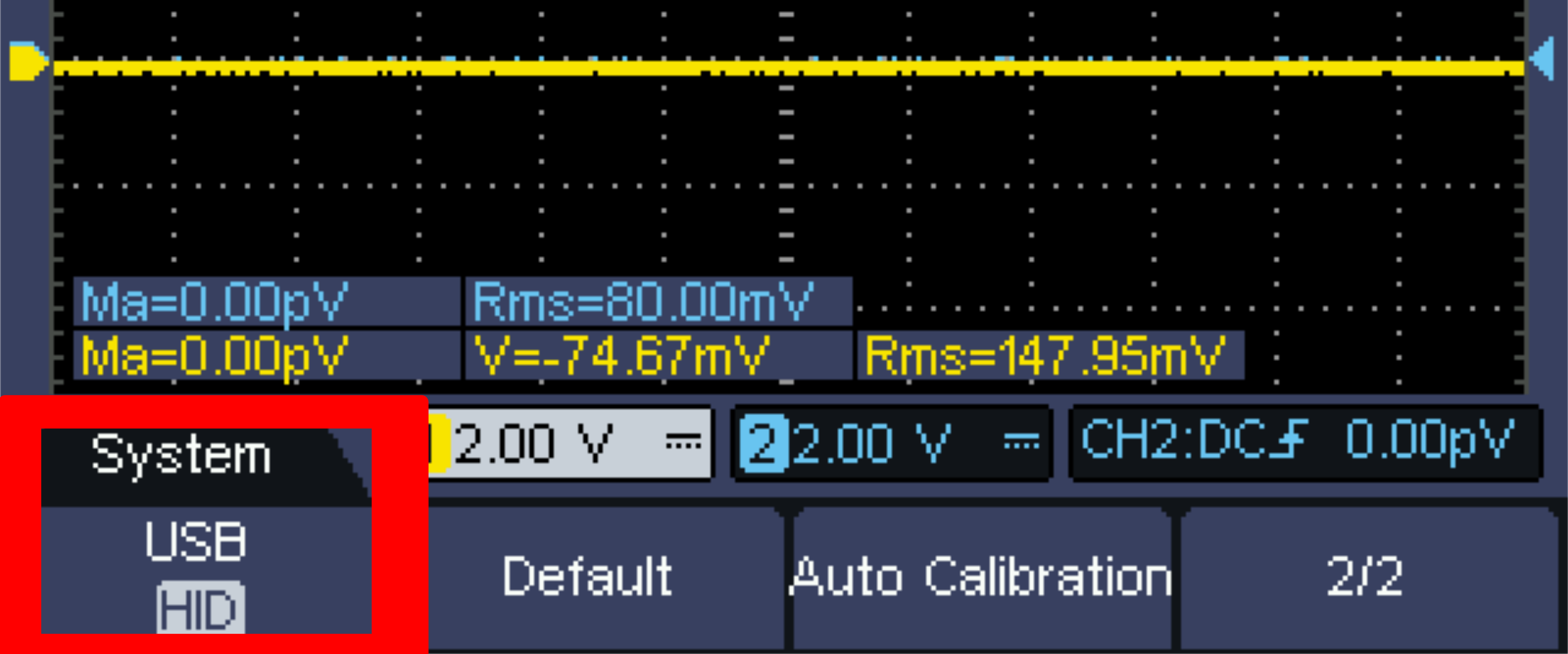
The Owon HDS25S supports SCPI commands over the USB port, and the HDS200(S) Series SCPI standard can be downloaded from Owon’s website (also from https://git.kloeckner.com.ar/hds25s/). To make the oscilloscope accept the SCPI commands the USB mode must be set to HID on the oscilloscope system settings, in this way when connecting it via USB, it reports as a serial device (on Linux based systems as /dev/ttyUSB*).

The cool thing about this oscilloscope is that it accepts SCPI commands for all of it three modes: multimeter, function generator and oscilloscope, and also that the function generator can be used at the same time as the oscilloscope. This last thing is a key point for achieving our goal.

Bode Plot

On a Bode plot, the magnitude and phase of the frequency response of a device is plotted as a function of frequency, with the frequency logarithmically spaced and the magnitude typically scaled in decibels. To achieve a bode plot, the traditional way is to connect a frequency generator on the input of the device under test (DUT for now on) and vary the frequency of the function generator, measuring and writing down the amplitude of the output of the DUT for every frequency.

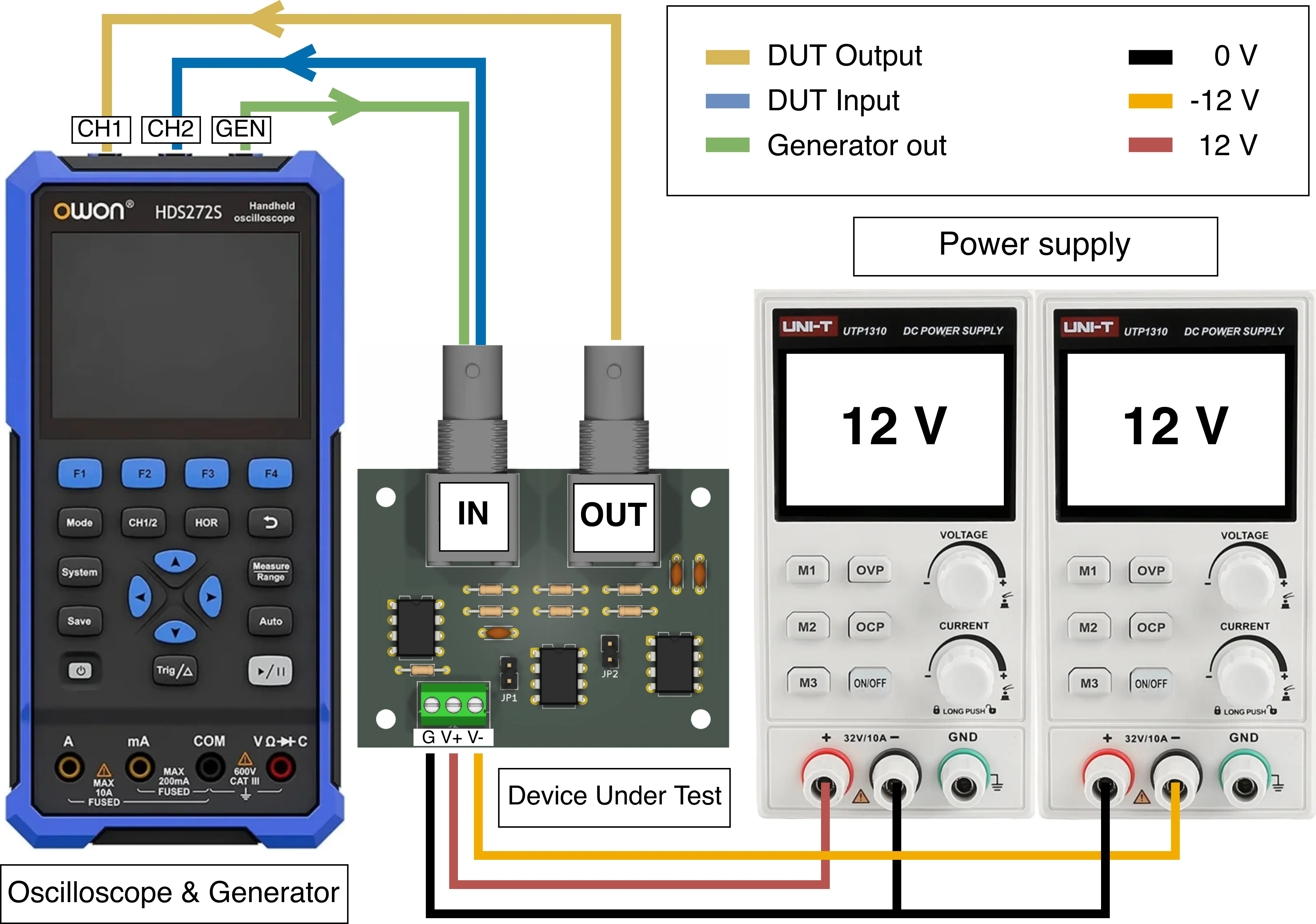
Given that the HDS25S supports SCPI commands for both the function generator and the oscilloscope, the connections for the automated and traditional methods are the same. The difference is that, instead of varying the frequency and measuring the output manually, SCPI commands are used. Consider the test bench shown below.

To automate the process of varying the frequency and measuring the output, a script is used. To obtain the magnitude data, the script must iterate over a list of logarithmically spaced frequencies and for every frequency do the following:

1. Set the function generator to the current frequency.
2. Measure the peak value of the output of the DUT.
3. Save the current frequency and the measured value on a list of results.

For example, consider the following pseudo-code.

frequencies = [1 10 100 1e3 10e3 100e3]
magnitude = []

for frequency in frequencies:
    func_generator.set_freq(frequency)
    measured_val = scope.measure_peak_val()
    magnitude.append(measured_val)

Getting the Data with PyVISA

The script used is written in Python using the PyVISA library to send and receive SCPI commands to and from the instrument. The PyVISA library abstracts away the communication interface used by the instrument (RS-232, USB, Ethernet, etc.), making it easy to establish communication with the instrument.

To use PyVISA, we need to know the device location beforehand. On Linux-based systems, the Owon HDS25S appears as /dev/ttyUSB* (when USB mode is set to HID, as mentioned). Knowing the device location, the following snippet sends the identification query. If everything is good the console should print the device response, for example “OWON,HDS25S,24531234,V8.8.2”.

import pyvisa

DEV_PATH="/dev/ttyUSB0"

rm = pyvisa.ResourceManager('@py')
dev = rm.open_resource(f"ASRL{DEV_PATH}::INSTR")
print("Identification: ", dev.query("*IDN?"), end="")

If the previous snippet worked it means that commands can be sent to and received from the instrument. To configure the oscilloscope, the folloing commands sets the channel 1 scale to 2 V per division, DC coupling and probe attenuation to X10.

dev.write(":CH1:SCALe 2.00V")
dev.write(":CH1:COUPling DC")
dev.write(":CH1:PROBE 10X")

Similarly for the function generator, the following sets the output to a sinusoidal wave with 1 V peak value and 1 kHz of frequency.

dev.write(":FUNCtion:AMPLitude 1.00")
dev.write(":FUNCtion SINE")
dev.write(":FUNCtion FREQuency 1000")

To vary the frequency, a list of logarithmically spaced frequencies is needed to iterate over. For this, the NumPy library and its logspace function are used to create the freqs list. An empty list amps is also created to append the measured amplitudes.

import numpy as np

freqs = np.logspace(0, 5, num=20)
amps  = []

Given the list of frequencies freqs, the following snippet steps through every frequency, setting the function generator to that frequency. After a small time delay, the peak value of the channel to which the output of the DUT is connected is measured and appended to the list of measured amplitudes amps. The time delay is needed because the measurement function of the scope is not instant after setting a new frequency.

for freq in freqs:
    scope.write(f":FUNCtion:FREQuency {freq}")
    tb_str = get_best_timebase(freq)
    scope.write(f":HORizontal:SCALe {tb_str}")
    time.sleep(0.5)
    val = float(scope.query(":MEASurement:CH1:MAX?").strip())
    amps.append(val)

The function get_best_timebase(freq) returns the best horizontal scale for the given frequency freq. Note that the peak value is measured using the channel 1 voltage ‘max’ measurement, equivalent to the voltage ‘max’ measurement from the physical menu. This has the disadvantage that the waveform must fit within the visual area to obtain the actual value. If it does not fit, the measurement returns, for example, “>10.00”, meaning that the peak value is greater than 10 volts and cannot be measured. A fix for this is to write a function similar to get_best_timebase, but for the vertical channel scale, setting the best fit for the vertical view space.

Plotting the Data

To get a figure of the Bode plot from the data we can use a python plotting library, for example matplotlib. Another possibility it to export the data and use another tool. I like Octave which is similar to MATLAB. To export the data as CSV consider the following snippet.

data = np.column_stack((freqs, amps))
np.savetxt("data.csv",
           data,
           delimiter=",",
           fmt=["%d", "%.2f"])

In Octave, plotting the data read from the CSV file is easy. In the following snippet, after loading the data, the measured values are normalized. This is achieved by dividing all the values by the function generator peak value (the peak value set in the function generator). Next, the values are converted to decibels, given that the values are voltage measurements, the conversion is done by taking the base 10 logarithm of every value times 20. Lastly, and optional, to smooth the curve a mean between contiguous values can be calculated using the movmean function, in the following snippet the mean is taken for every 5 contiguous values.

data = csvread("data.csv");
freq = data(:, 1);
mag  = data(:, 2);

mag_db = 20 * log10(mag);
mag_db_smooth = movmean(mag_db, 5);

figure();
semilogx(freq, mag_db_smooth);

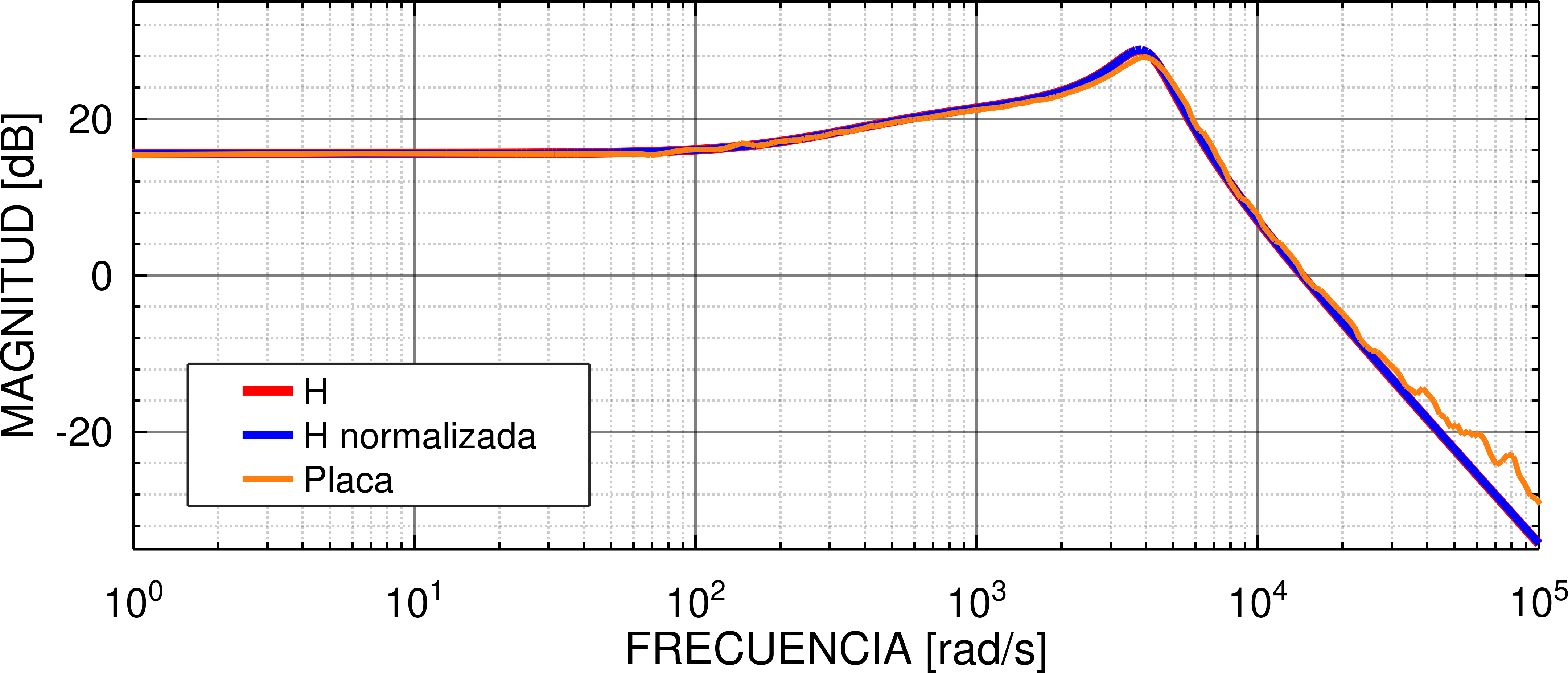
In a similar manner as above but tweaking the appearance of the figure, the following bode plot is obtained. The orange trace represents the frequency response obtained with this method. The red trace, “H”, is the frequency response of the theoretical transfer function of the DUT. The blue trace, “H normalizada”, is the frequency response of the theoretical transfer function of the DUT but with normalized commercial component values.